Anomaly detection with Autoencoders

In my recent studies on computer vision and machine learning, I came across the concepts of autoencoders. Essentially, Autoencoders are neural networks which are trained using unsupervised learning.

The aim of training an autoencoder is to learn a compressed representation of a given input. Internally, the network is able to learn the salient features of the data through successive layers and compresses it into a latent space representation. In some ways, this is similar to other algorithms such as PCA.

The learned compressed latent space representation can be used in areas such as dimensionality reduction; denoising; and anomaly detection, which is the focus of this post.

An autoencoder consists of 2 main components: encoder, decoder. The encoder is responsible for learning a latent representation of the input. The decoder tries to reconstruct the original input from the learned latent space.

While there are speciality algorithms for anomaly detection such as IsolationForests; DBScan; and RCF, we will attempt to construct and autoencoder using tensorflow.

Since we are dealing with image inputs, we can build a convolutional autoencoder. The model will comprise of convolutional layers which downsamples the input in the encoder model; and convolutional transpose layers to upsample the input in the decoder model to reconstruct the latent representation back into its original dimension.

An example autoencoder could be as follows:

1
2
3
4
5
6
7
8
9
10
11
12
13
14
15
16
17
18
19
20
21
22
23
24
25
26
27
28
29
30
31
32
33
34
35
36
37
38
39
40
41
42
43
44
latent_dim = 16

input_shape = (height, width, depth)
chan_dim = -1

if K.image_data_format() == "channels_first":
	input_shape = (depth, height, width)
	chan_dim = 1

inputs = Input(shape=input_shape)
x = inputs

# Build encoder
for f in filters:
	# use strided convolutions to downsample
	# no pooling layers...
	x = Conv2D(f, (3,3), strides=(2, 2), padding="same")(x)
	x = LeakyReLU(alpha=0.2)(x)
	x = BatchNormalization(axis=chan_dim)(x)

vol_size = K.int_shape(x)
x = Flatten()(x)
x = Dropout(0.5)(x)
latent = Dense(latent_dim)(x)
encoder = Model(inputs, latent, name="encoder")

# Decoder which accepts output of encoder as input
latent_inputs = Input(shape=(latent_dim,))
x = Dense(np.prod(vol_size[1:]))(latent_inputs)
x = Reshape((vol_size[1], vol_size[2], vol_size[3]))(x)

for f in filters[::-1]:
	# apply CONV_TRANSPOSE => RELU => BN
	x = Conv2DTranspose(f, (3,3), strides=(2,2), padding="same")(x)
	x = LeakyReLU(alpha=0.2)(x)
	x = BatchNormalization(axis=chan_dim)(x)

# apply single conv transpose layer to recover original depth of image
x = Conv2DTranspose(depth, (3,3), padding="same")(x)
outputs = Activation("sigmoid")(x)

decoder = Model(latent_inputs, outputs, name="decoder")

autoencoder = Model(inputs, decoder(encoder(inputs)), name="autoencoder")

Normally in a typical CNN model, we use MaxPooling to downsample the input dimensions. In this case, we are using strides of 2 to reduce the dimensions by half. By the fully-connected layers of the Encoder model, the input is reduced down to the specified latent_dim of 16.

For the decoder, we use a convolutional transpose to upsample the latent dimension back to its original size. The outputs are then passed through a sigmoid activation layer as we have scaled our image inputs to be in the range of [0,1].

The two models are then used to construct the autoencoder model which is the model used for training and evaluation. Note that in the output of the autoencoder model, we specified the following:

1
  decoder(encoder(inputs))

Since our aim is to train a model to reconstruct the inputs, it follows that we want our model to learn the following scoring function, given X as input:

1
  f(X) = D(E(X))

From my own experimentation, I found that most of the articles or books I came across use MNIST as the dataset, which is in grayscale.

It can be difficult to train an autoencoder in RGB images as they are of higher dimensionality with 3 colour channels. I had to make the following alterations to the training process as follows:

• Increased the number of epochs to at least 100

• Increased the latent dimensionality of model to be at least 128

• Use a high learning rate to start training and gradually reduce it using weight decay

• Given the small number of training images, I used the ImageDataGenerator to augment the training set. I also used dropout and weight decay on the model to combat overfitting.

The loss function was defined to the mean-squared-error(MSE) between the original image and the reconstructed image. During evaluation, we compute the MSE as the reconstruction loss and the lower the loss, it means the model has learnt a useful latent representation of the inputs and is able to reconstruct it.

For this given example, I have trained the autoencoder model on 328 RGB images of forests, with 20% for validation. For the test set, I gathered some random images which don’t contain any forest imagery and evaluated its MSE.

A loss plot of the training process is shown below:

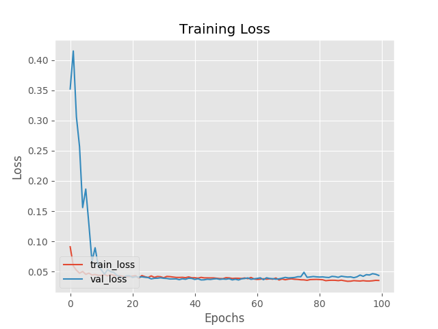
Both the training and validation loss curves show convergence from epoch 10 onwards. However, there is still overfitting from epoch 70 onwards as the validation loss starts to rise. The final reconstruction loss is 0.04396.

A sample of the reconstruction from the final autoencoder is shown below:

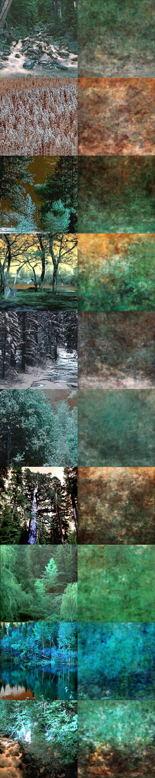
The images in the left column show the original images and the right show the reconstructed images. The reconstructed image resolution is not as clear but the model is able to capture the salient features such as the green hues and tree like shapes, which are in forest imagery.

The complete code repository can be found here.

Keep hacking and stay curious!